How to use PhyTA

Comparing phylogenetic trees

To start using PhyTA we need to go to the processing page by clicking in the Process menu available in the navigation bar.

Figure 1.1: PhyTA’s navigation bar.

To add a new phylogenetic tree for process we use the text area below, as in Figure 1.2. Note that only one tree must be added at a time.

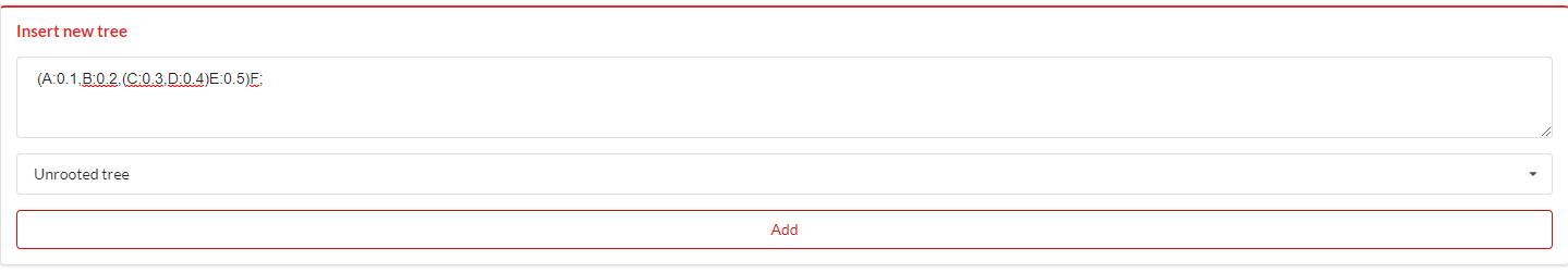
Figure 1.2: Adding a new tree.

For example, we will add two trees: (A:0.1,B:0.2,(C:0.3,D:0.4)E:0.5)F; and (X:0.1,B:0.2,(C:0.3,D:0.4)E:0.5)F; one at a time. The trees added will appear in the table above as in Figure 1.3. After adding the trees the user needs to specify the metrics to use for comparison. All trees will be compared to one another using all the metrics chosen. Not all metrics are suitable for certain tree types. When the user chooses a metric that is not suitable for some tree type this metric will not be processed.

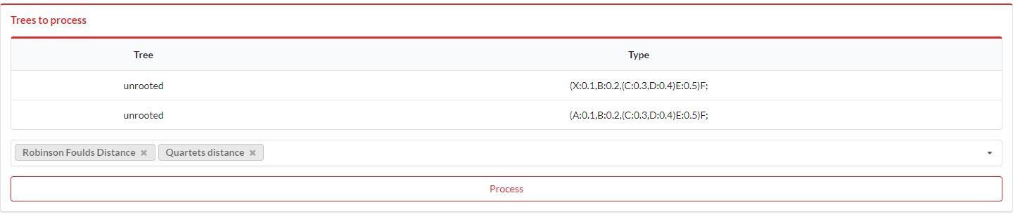
Figure 1.3: Trees added.

After putting the trees for process a modal will appear with the processing job id.

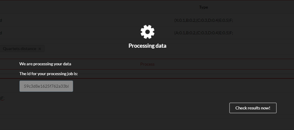
Figure 1.4: Modal with the processing job id.

The user can check the results by clicking the Check results now! button or by navigating to the Results menu in the navigation bar.

Visualizing the results

The user can later visualize the processing job results by clicking the Results menu in the navigation bar. The the user can insert the processing job id like in Figure 1.5.

Figure 1.5: Inserting the processing job id.

Then, a matrix table with the metric results will appear as in Figure 1.6. The user can export these results by clicking in the exports button. A JSON file will be downloaded containing information about the trees and all the comparison results.

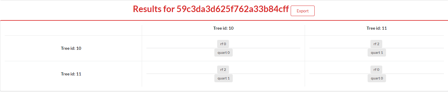
Figure 1.6: Matrix table with the metric results.

If the user wants to see the differences between the trees visually they can click a result and a side by side comparison of the trees will appear as in Figure 1.7.

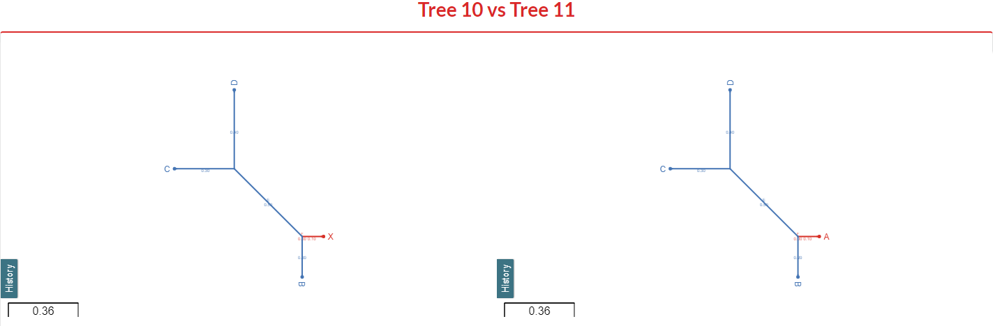
Figure 1.7: Side by side comparison of two trees.

Interpret the differences

It is important to clarify that the painted differences vary according to the metric being visualized.

Figure 1.8: Marking the differences.

When comparing two trees side by side the similarities or dissimilarities of the two trees will be displayed using a color scale.

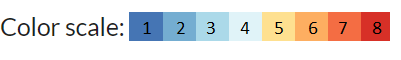
Figure 1.9: Color scale.

Legend for the color scale:

• 1 - Equal
• 2 - Most similar
• 3 - Most dissimilar
• 4 - Different

The branches and nodes for both trees are painted according to the differences processed and which differ according to the metric being visualized.

Authentication

The user can authenticate via Google and has the option to see all the processing job ids requested by him as in Figure 1.7. When a processing job results are ready the user will receive an email.

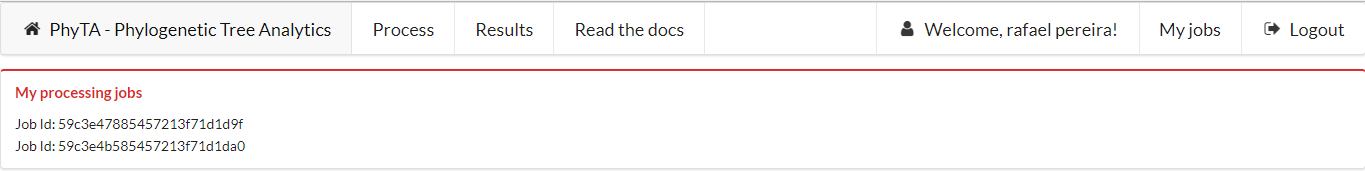
Figure 1.7: My Jobs menu for authenticated users.